NIST RESEARCH PROJECTS
Overview
The mmWave imaging system consists of visualizing images by recording mmWaves scattering off of objects.
Old System
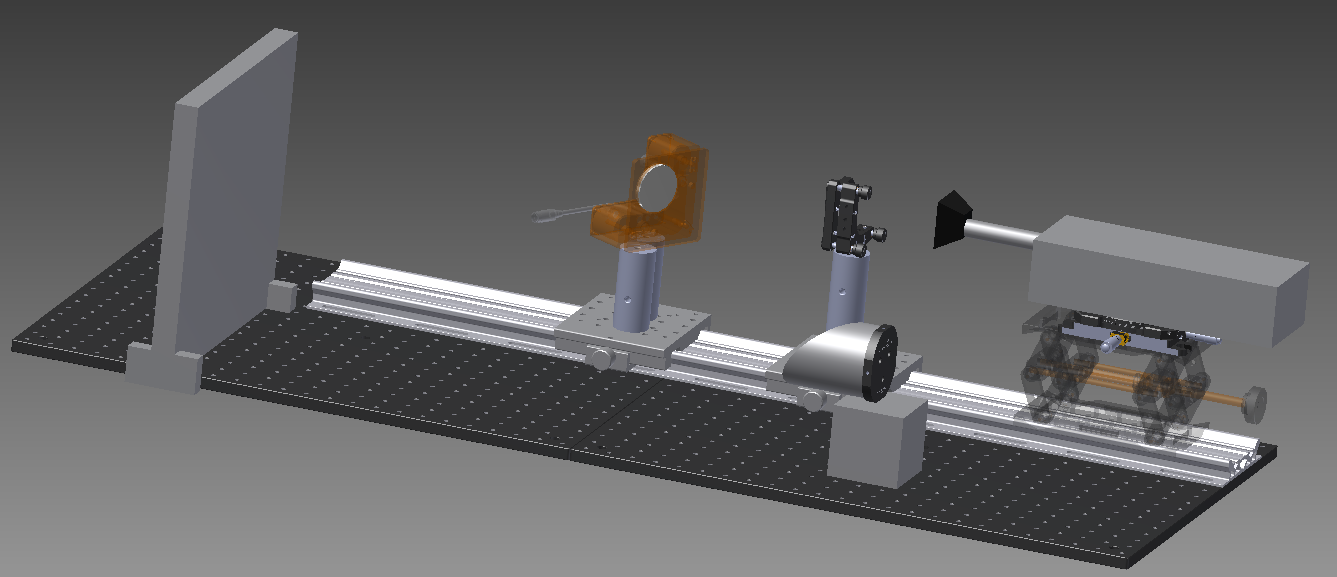
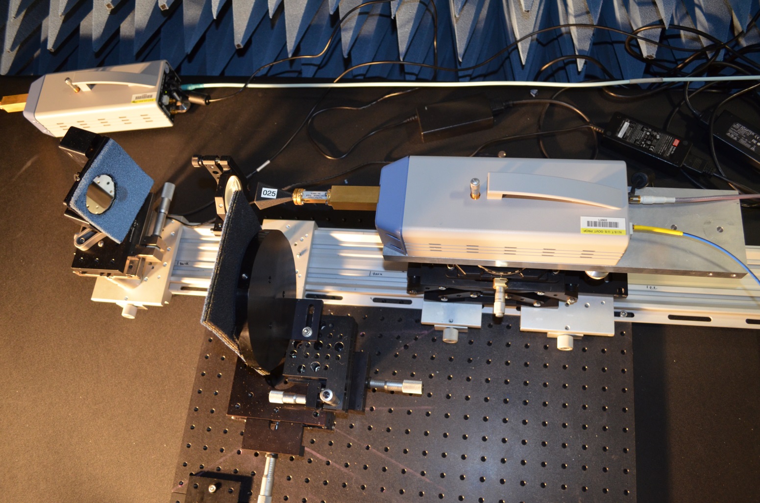
I set up a scanning system that drives a beam to point along a grid, and measures the power produced by Radio Frequency (RF) energy scattering off the object at each point. First the emitting frequency converter shines RF energy on a motorized mirror that is then reflected off of another stationary mirror toward the object desired to be imaged. The receiving frequency converter then takes in the reflected RF energy off of the object. The motorized mirror then moves and another RF intensity point is collected scanning through a whole xy grid. This setup is shown in the two images to the right.
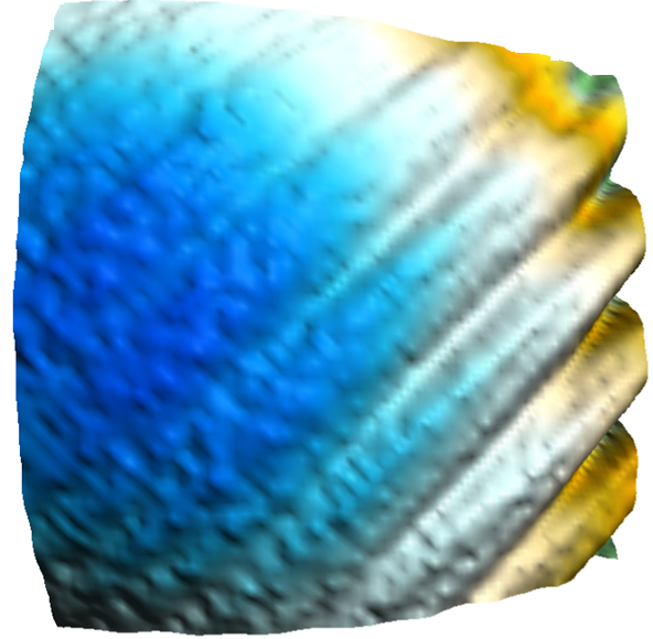
Results
A few results of the mmWave images created by processing the scan data are shown to the right.

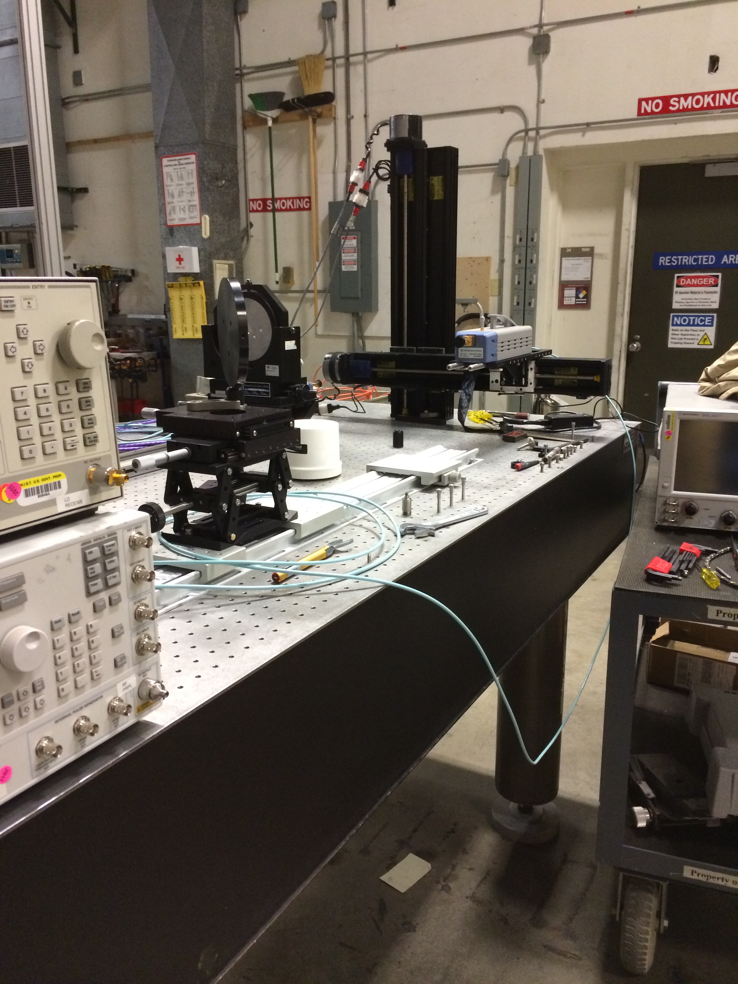
New System
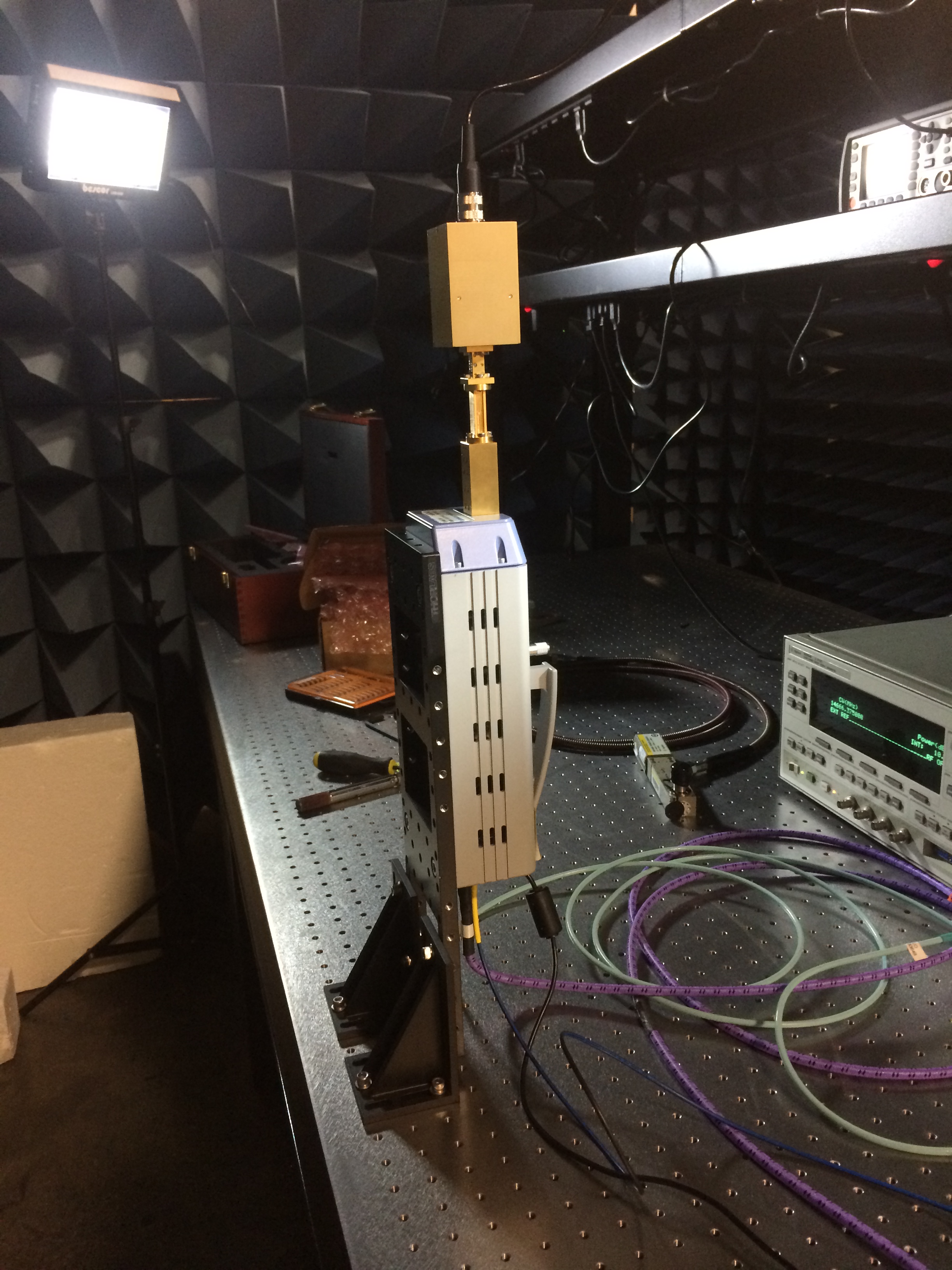
To improve the previous work we added an x-y stage to control the position of the emitting frequency converter while keeping the mirror stationary to improve alignment. Also, with the frequency converter on the x-y stage we were able to do an electrical alignment instead of a laser alignment. As well, the new set-up involves just one mirror to project the radiated RF energy.

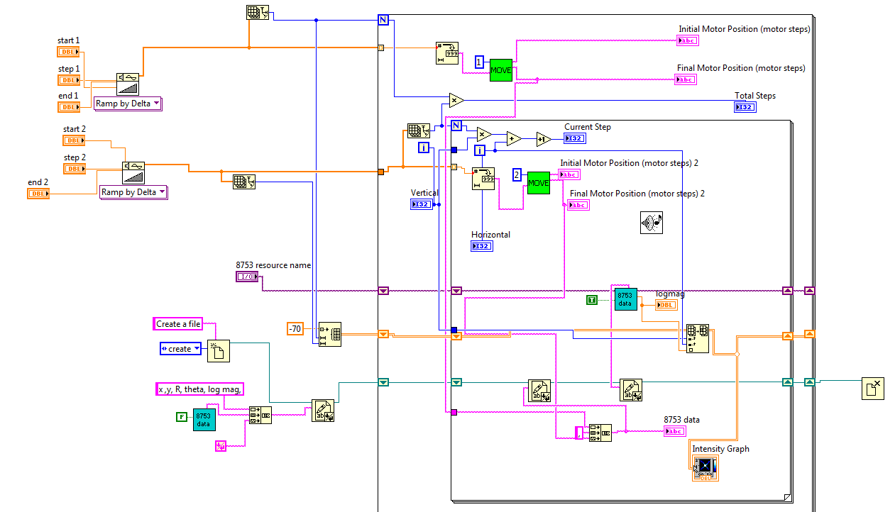
New System Code
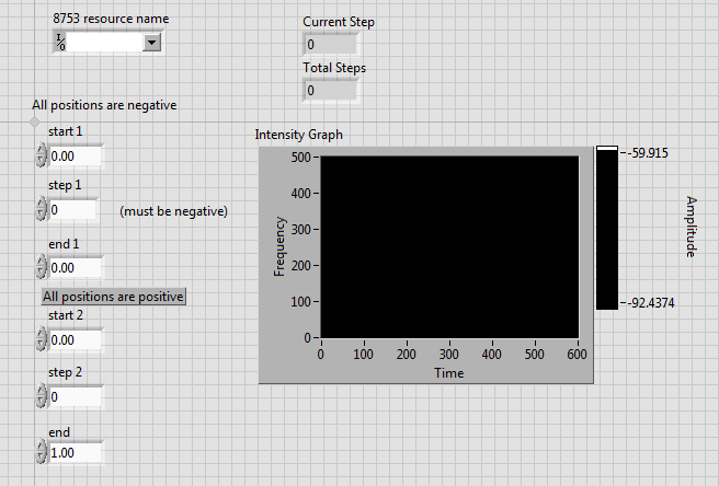
The code I generated drives the motor over a specified x-y grid and measures RF energy at each point on the grid. Next the data was read into MATLAB and a 2D Fourier Transform was performed to generate the image.
Overview:
I created an automated system of a 90-140 GHz power reference. This allowed us to establish a stable reference output power used to calculate electric field linearity for atomic based field probe research. The system consisted of a frequency converter connected to two signal generators (SGs), a spectrum analyzer (SA), a mmWave power meter and a RF power meter. The figure to the right shows the set up of the frequency converter connected to a power meter to regulate and control power levels. The frequency converter multiplies the frequency of SG1 to generate the mmWave power signal and uses SG2 to down-convert a portion of the signal to a detectable frequency. Both SGs are needed to generate a +7 dBm signal at the correct frequency. The RF power meter reads the output of the SGs and the SA measures the sampled signal.
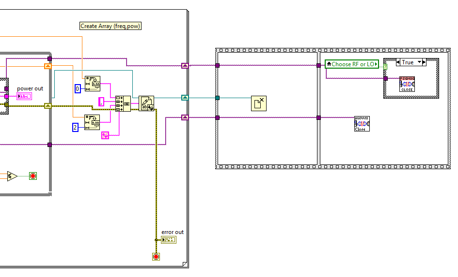
Initialize:
First the power levels needed to be set for the SGs. This was done by hooking up a RF power meter to the SGs and running a LabView vi to find the calibrated power needed to reach the manufacturer specified +7dBm output power level at the LO and Rf inputs to the frequency converters. As well, the code generated a power level reference spreadsheet from these values. The code below shows the process of implementation of finding the needed output power within a tolerance of .1 dB.
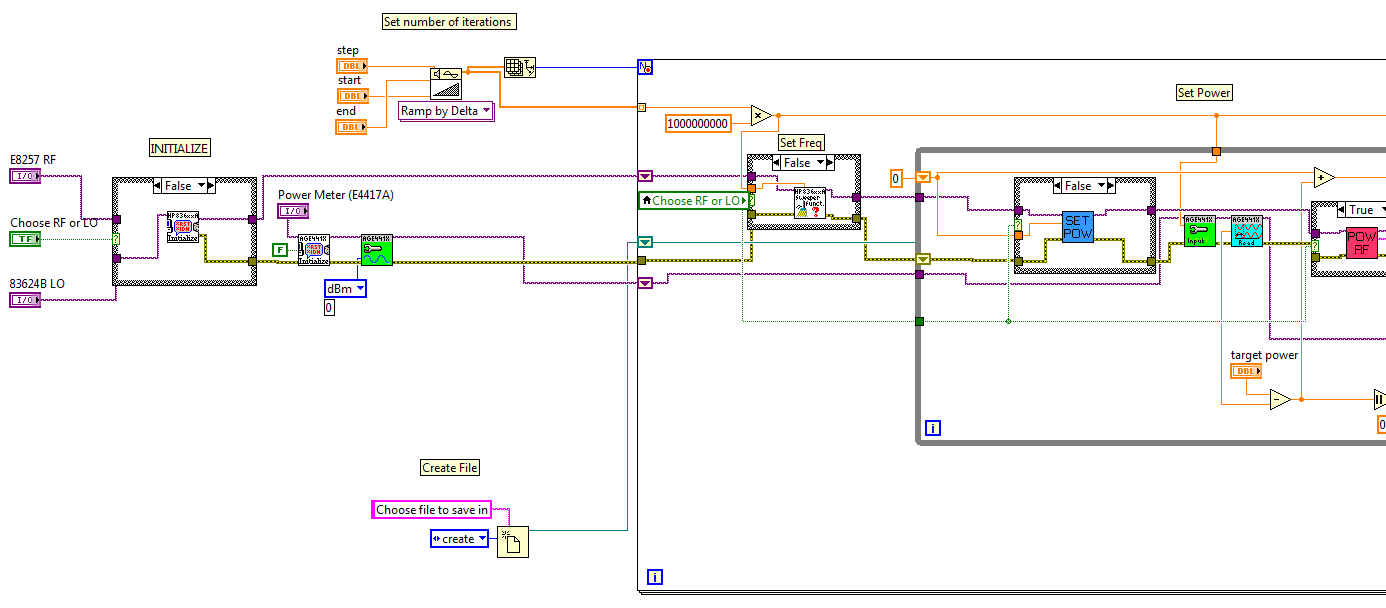
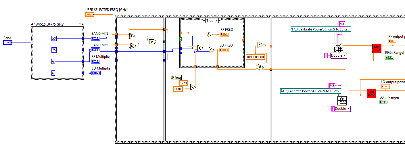
The Process:
With the generated spreadsheet above I wrote another LabVIEW vi to calculate the power needed to be sent to the generators for a selected frequency in a specified bandwidth. This is done by directly measuring the frequency converter output with the mmWave power meter. This is then compared with the sampled power measured by the SA (from the spreadsheet). This allows the output power of the converter to be inferred from the SA without the mmWave power meter. The final result is a an adjustable calibrated power source across 90-140GHz frequency range. The code below shows this process.
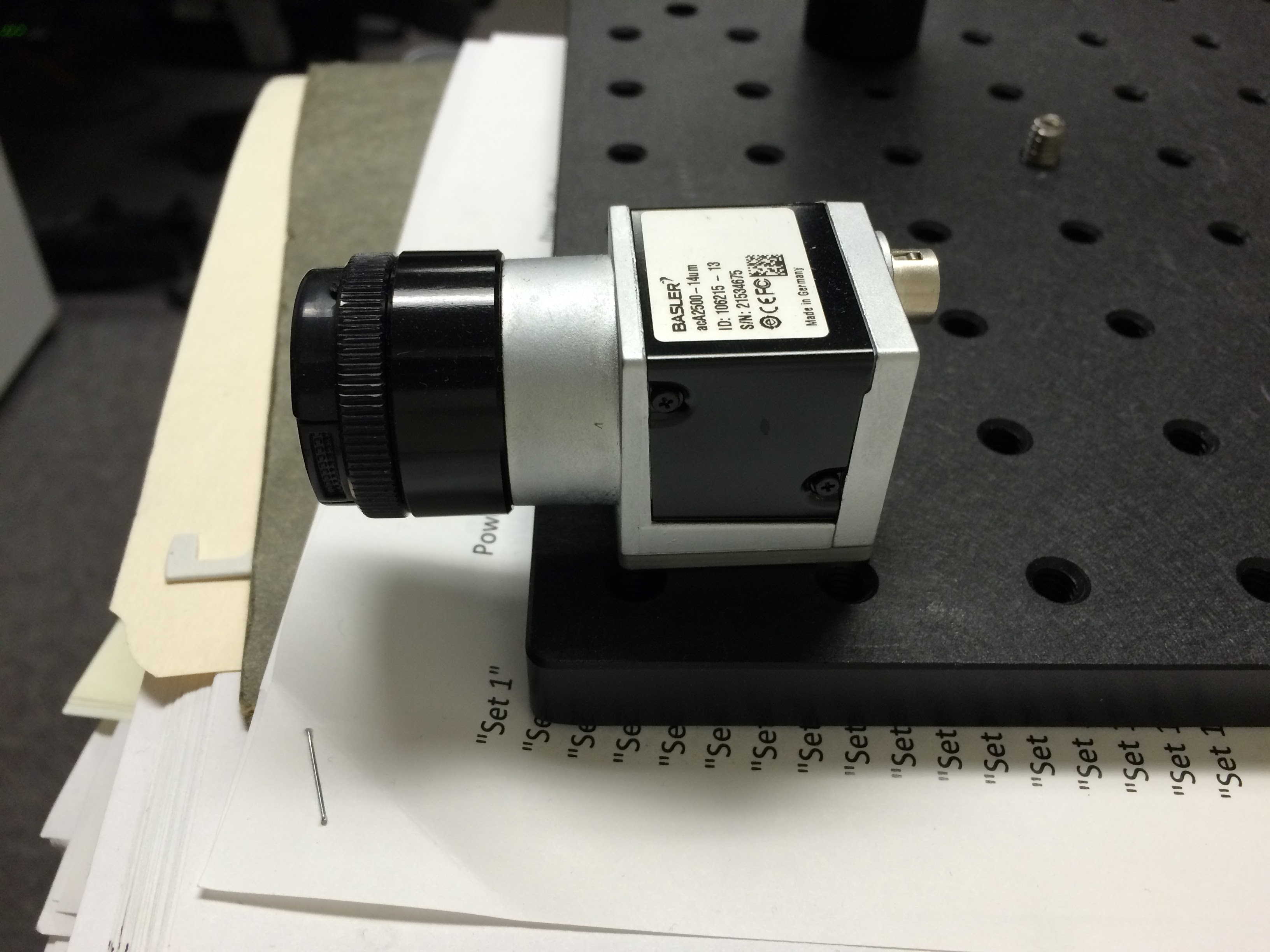
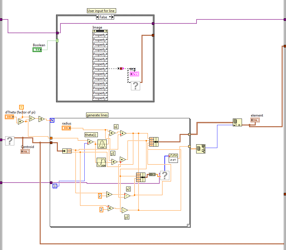
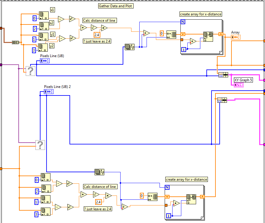
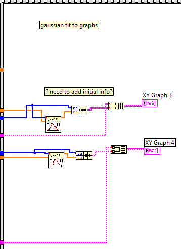
The laser beam profiler captures an image of a laser beam with a web cam (shown right) and finds characteristics of the laser beam through a Gaussian fit model via LabView code I developed. The code (shown below) consists of creating perpendicular lines through the width and height of the imaged oval shaped beam. This is done by scanning through the image with lines and finding the line that has the maximum value of intensities and making a perpendicular line to that line. The intensity values across these lines allow for characteristics of the beam to be found through the Gaussian fit model.